You don't have to be a professional data analyst or an accountant to benefit from some of the basic tools and functions in Microsoft Excel. As businesses and organizations become more reliant on data and information systems to make decisions, more employees must interact with data on a daily basis. According to a recent report by Burning Glass Technologies, which was the subject of an article in the Wall Street Journal - The Key to a Good-Paying Job Is... Microsoft Excel?, learning Microsoft Excel and other basic digital skills is essential to getting a job that promises a living wage and a good shot at a middle-class life.

This is the first of a series of blog posts that will demonstrate how to use some of the basic tools available in Microsoft Excel so that you can become more proficient. I want to start by introducing the use of Excel tables. There are many benefits to using Excel tables in lieu of a plain data set. Here are a few:

Data becomes easier to read by adding alternating colors with banded rows or banded columns.
Data in any column can be easily sorted in ascending or descending order.
Data in any column can be easily filtered so that you only see the data you want to see.
Totals can easily be added for each column, such as sum, average, count, and more.
Always see the column names no matter how far down you scroll in the spreadsheet.

Creating an Excel Table

Here is a basic data set, consisting of a few hundred rows of transactional data. In order for a data set to be converted into an Excel table there can be no blank columns or rows and ideally, each column has a column heading that describes the data in each column.

Keyboard Shortcut

There are a couple of ways to convert a data set, like this one, into a table. The easiest of which is by completing the following steps:

Click any cell inside the data set.
Press Ctrl + T on the keyboard

This keyboard shortcut will bring up the Create Table dialog box identifying the range selected and a check box for indicating whether or not your data has column headers.

Once you click OK in the Create Table dialog box, your data set will be converted to an Excel table. Let the reaping of the benefits begin!

Customize a Table

If you now look to the Ribbon, assuming you did not select a cell outside of the data set, you will see a new contextual tab labeled TABLE TOOLS - DESIGN. This tab provides you with several different options to customize your table. Let's begin with the group of options labeled Table Style Options.

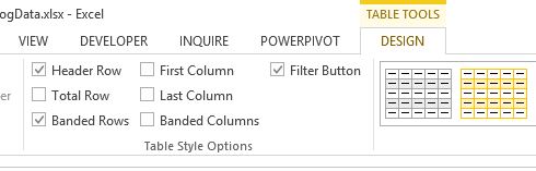
By default, an Excel table is formatted with Banded Rows, Filter Buttons, and if indicated in the Create Table dialog box, a Header Row. Checking the First Column or Last Column check boxes adds a bold font style to the data in each of the respective columns. Checking the Total Row check box will add a row to the bottom of the table with access to any Excel function to summarize the data in each column. Similar to the Banded Rows, checking the Banded Columns check box will alternate the colors of the columns in the table.

Apply Table Styles

Also on the TABLE TOOLS - DESIGN tab is a group labeled Table Styles.

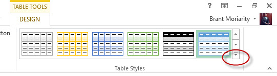
If you are not a fan of the default table style, you can select from a variety of built-in options. Click the more arrow, circled above, to view more options and to reveal the option to create a new table style.

Format as Table

Instead of using the keyboard shortcut mentioned above to create a table, after clicking any cell inside the data set you can click the Format as Table button located in the Styles group on the HOME tab to select a style and create a table simultaneously.

Sort and Filter

Now that you know how to create a table and select a table style, let's take a look at how to use the table to sort and filter. Assuming you have column headings and that the default Filter Buttons is checked, you will see an arrow to the right of each column heading.

Clicking the arrow will reveal the sort and filter options for that particular column. This allows you to easily view your data from highest to the lowest or vice versa. It also allows you to view specific records by utilizing the filters.

Using Table Totals

If you checked the Totals check box in the Table Style Options group, you can scroll down to the final row and explore this feature. As you scroll down, you'll notice that the column headings remain visible This is very useful!

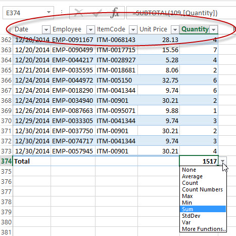
The Total row give you an option to select from a list of commonly used functions to summarize each of the columns. The great thing about these functions is that if you filter your data to only view certain records, the calculations will only occur on the records that are visible. To accomplish this, Excel will automatically insert the SubTotal function when you select one of the aggregate functions from the list.

Adding Columns and Formulas

Another benefit of using Excel tables is the ability to easily add new columns of data that automatically become part of the table. Since our data set has unit price and quantity columns we can now easily calculate revenue in a new column. Typing a new column heading to the right of the Quantity column, automatically adds that column to the table.

We can now enter a revenue calculation in cell F2 by typing =D2*E2. As you click each cell reference in the table, Excel will convert the cell address to a table reference. So, =D2*E2 becomes =[@[Unit Price]]*[@Quantity]. Once you press Enter, the same formula will be entered in every row down the column. The table formulas add clarity to your calculations by utilizing the column headings and having the formula automatically entered down the entire column can save you quite a bit of time and ensures consistency.

Blog

View, Sort, and Filter Data with Excel Tables